

How To Draw A Data Model
Model basics
Introduction
The goal of a model is to provide a unproblematic low-dimensional summary of a dataset. In the context of this book we're going to use models to partitioning data into patterns and residuals. Strong patterns will hide subtler trends, so nosotros'll employ models to assist peel back layers of structure as nosotros explore a dataset.
Notwithstanding, before we tin first using models on interesting, real, datasets, you need to sympathise the basics of how models work. For that reason, this affiliate of the book is unique because it uses only simulated datasets. These datasets are very simple, and not at all interesting, but they volition help yous empathize the essence of modelling before you apply the same techniques to real data in the next chapter.
At that place are 2 parts to a model:
-
Showtime, you define a family of models that express a precise, but generic, design that yous desire to capture. For example, the pattern might exist a straight line, or a quadratic curve. You volition express the model family equally an equation like
y = a_1 * x + a_2ory = a_1 * ten ^ a_2. Hither,xandyare known variables from your data, anda_1anda_2are parameters that can vary to capture unlike patterns. -
Adjacent, y'all generate a fitted model by finding the model from the family unit that is the closest to your data. This takes the generic model family and makes it specific, similar
y = 3 * 10 + 7ory = nine * x ^ 2.
Information technology's of import to understand that a fitted model is merely the closest model from a family unit of models. That implies that y'all accept the "best" model (co-ordinate to some criteria); it doesn't imply that y'all accept a good model and it certainly doesn't imply that the model is "true". George Box puts this well in his famous aphorism:
All models are incorrect, but some are useful.
It'south worth reading the fuller context of the quote:
Now it would be very remarkable if any system existing in the existent world could be exactly represented past any unproblematic model. Even so, cunningly chosen parsimonious models oft practise provide remarkably useful approximations. For example, the law PV = RT relating pressure P, volume V and temperature T of an "ideal" gas via a constant R is non exactly true for whatsoever existent gas, simply information technology frequently provides a useful approximation and furthermore its structure is informative since it springs from a physical view of the behavior of gas molecules.
For such a model there is no need to ask the question "Is the model true?". If "truth" is to be the "whole truth" the answer must be "No". The but question of interest is "Is the model illuminating and useful?".
The goal of a model is not to uncover truth, only to find a unproblematic approximation that is still useful.
Prerequisites
In this chapter we'll utilise the modelr package which wraps effectually base R's modelling functions to brand them work naturally in a pipe.
A uncomplicated model
Lets have a look at the simulated dataset sim1, included with the modelr package. It contains two continuous variables, 10 and y. Let'south plot them to see how they're related:
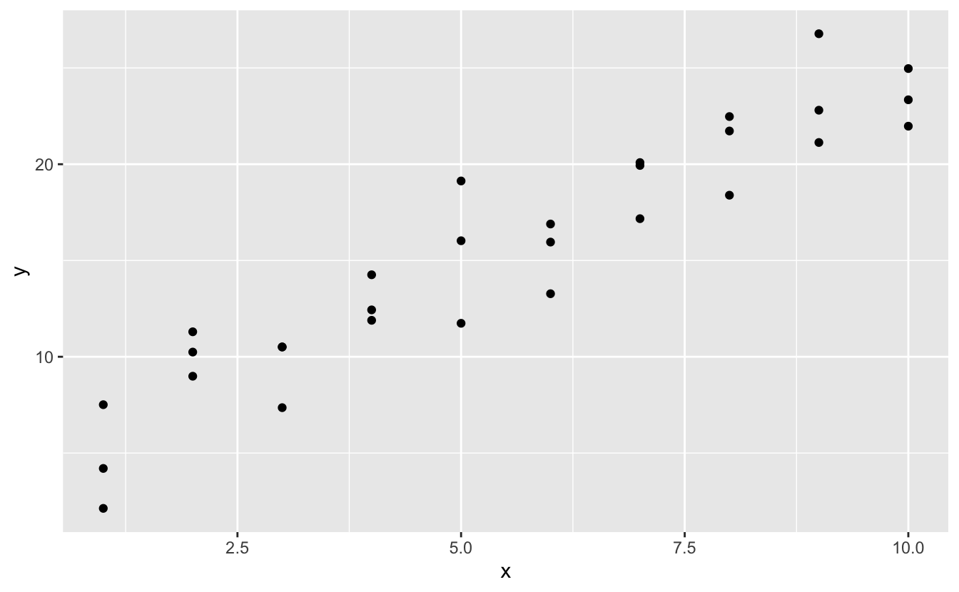
You can encounter a potent pattern in the data. Allow'due south use a model to capture that pattern and brand it explicit. It's our job to supply the bones grade of the model. In this case, the relationship looks linear, i.e.y = a_0 + a_1 * 10. Allow'due south beginning past getting a experience for what models from that family look similar past randomly generating a few and overlaying them on the data. For this simple example, we can use geom_abline() which takes a slope and intercept as parameters. Later on we'll learn more general techniques that work with whatsoever model.
models <- tibble ( a1 = runif ( 250, - 20, xl ), a2 = runif ( 250, - 5, 5 ) ) ggplot ( sim1, aes ( x, y ) ) + geom_abline ( aes (intercept = a1, slope = a2 ), data = models, alpha = 1 / 4 ) + geom_point ( ) 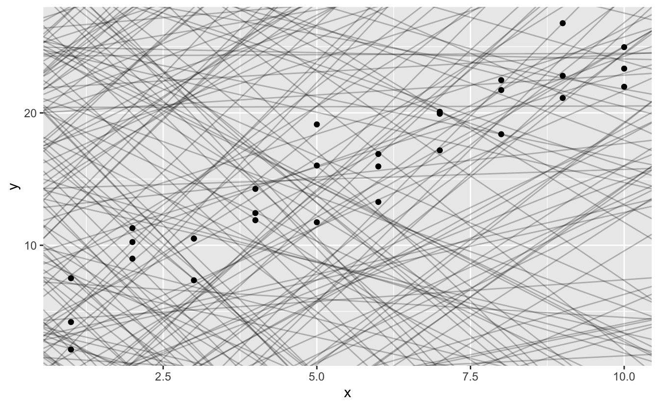
In that location are 250 models on this plot, just a lot are actually bad! We need to notice the skillful models by making precise our intuition that a good model is "close" to the data. Nosotros need a manner to quantify the distance between the data and a model. Then we can fit the model by finding the value of a_0 and a_1 that generate the model with the smallest altitude from this data.
One easy place to start is to find the vertical distance betwixt each point and the model, as in the following diagram. (Note that I've shifted the x values slightly so you lot can come across the individual distances.)
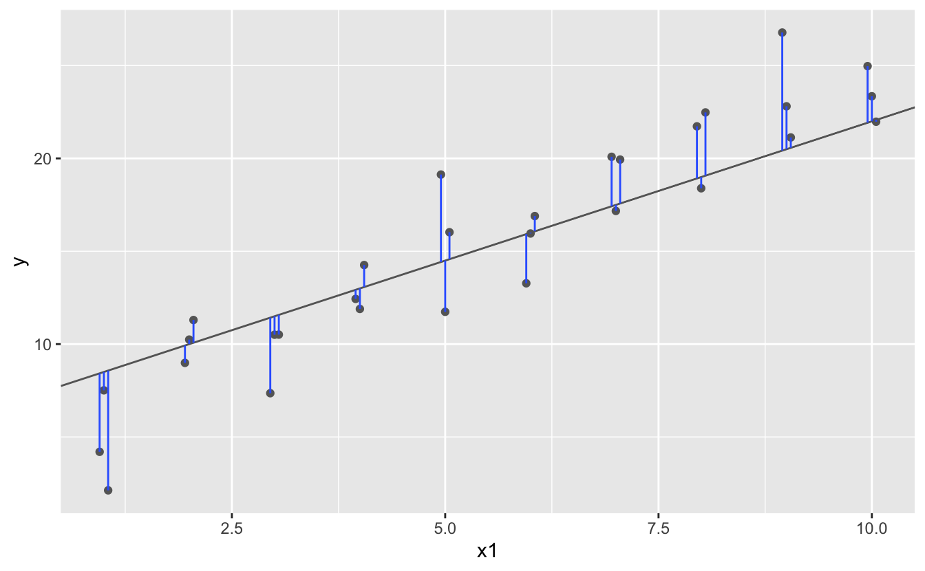
This distance is just the difference between the y value given by the model (the prediction), and the actual y value in the information (the response).
To compute this distance, we offset turn our model family into an R function. This takes the model parameters and the data every bit inputs, and gives values predicted by the model as output:
model1 <- function ( a, data ) { a [ 1 ] + information $ 10 * a [ 2 ] } model1 ( c ( 7, ane.5 ), sim1 ) #> [i] 8.5 viii.five 8.five ten.0 10.0 10.0 xi.v xi.5 11.five xiii.0 xiii.0 13.0 14.5 14.5 xiv.5 #> [16] 16.0 xvi.0 xvi.0 17.5 17.5 17.5 nineteen.0 xix.0 nineteen.0 20.5 20.5 20.5 22.0 22.0 22.0 Next, we need some way to compute an overall altitude between the predicted and bodily values. In other words, the plot higher up shows thirty distances: how do we plummet that into a single number?
1 mutual way to do this in statistics to use the "root-mean-squared departure". We compute the deviation between actual and predicted, square them, average them, and the take the square root. This distance has lots of highly-seasoned mathematical properties, which we're not going to talk nigh here. You'll just have to take my word for information technology!
measure_distance <- function ( mod, information ) { unequal <- data $ y - model1 ( modernistic, information ) sqrt ( mean ( unequal ^ 2 ) ) } measure_distance ( c ( 7, 1.5 ), sim1 ) #> [one] 2.665212 Now we can use purrr to compute the distance for all the models defined higher up. We need a helper office because our altitude function expects the model every bit a numeric vector of length 2.
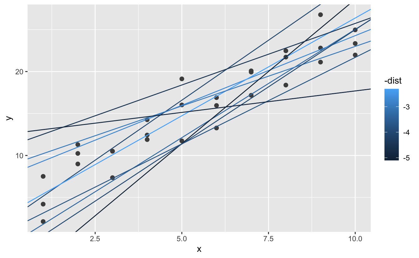
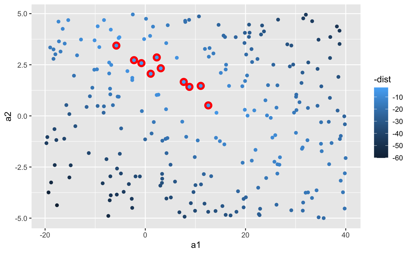
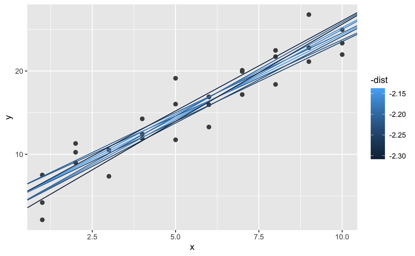
sim1_dist <- office ( a1, a2 ) { measure_distance ( c ( a1, a2 ), sim1 ) } models <- models %>% mutate (dist = purrr :: map2_dbl ( a1, a2, sim1_dist ) ) models #> # A tibble: 250 x iii #> a1 a2 dist #> <dbl> <dbl> <dbl> #> i -15.ii 0.0889 xxx.eight #> 2 30.1 -0.827 xiii.2 #> 3 16.0 ii.27 13.2 #> four -ten.vi 1.38 18.seven #> 5 -xix.vi -1.04 41.8 #> six seven.98 iv.59 19.3 #> # … with 244 more rows Side by side, let's overlay the 10 all-time models on to the data. I've coloured the models by -dist: this is an like shooting fish in a barrel way to make sure that the best models (i.due east. the ones with the smallest altitude) get the brighest colours.
We can also think nigh these models as observations, and visualising with a scatterplot of a1 vs a2, again coloured by -dist. We can no longer straight see how the model compares to the data, simply we can run into many models at once. Again, I've highlighted the 10 best models, this fourth dimension by drawing red circles underneath them.
Instead of trying lots of random models, we could be more than systematic and generate an evenly spaced grid of points (this is called a grid search). I picked the parameters of the grid roughly past looking at where the all-time models were in the plot above.
filigree <- expand.grid ( a1 = seq ( - five, 20, length = 25 ), a2 = seq ( 1, 3, length = 25 ) ) %>% mutate (dist = purrr :: map2_dbl ( a1, a2, sim1_dist ) ) grid %>% ggplot ( aes ( a1, a2 ) ) + geom_point (data = filter ( grid, rank ( dist ) <= x ), size = 4, colour = "reddish" ) + geom_point ( aes (color = - dist ) ) 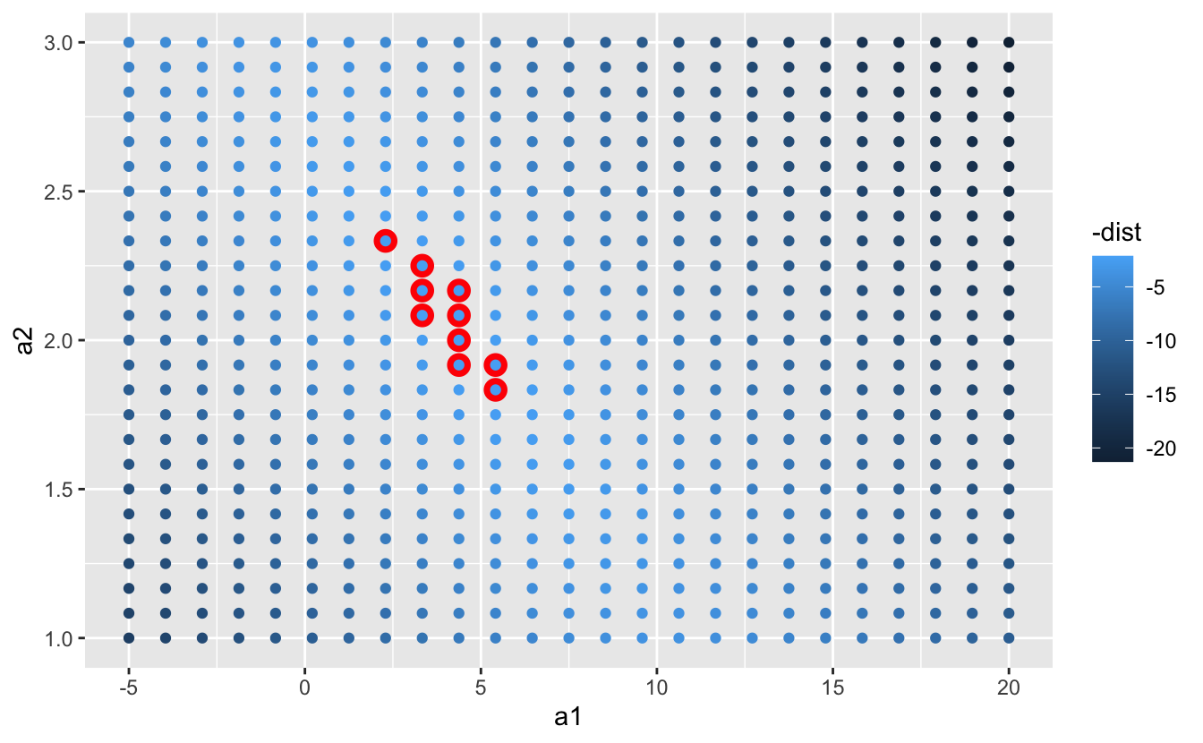
When y'all overlay the best 10 models back on the original data, they all await pretty expert:
Y'all could imagine iteratively making the grid finer and finer until you narrowed in on the best model. But there's a better way to tackle that problem: a numerical minimisation tool called Newton-Raphson search. The intuition of Newton-Raphson is pretty simple: yous pick a starting betoken and await around for the steepest slope. You lot then ski down that gradient a footling fashion, and and then repeat over again and over again, until y'all can't go any lower. In R, we can do that with optim():
best <- optim ( c ( 0, 0 ), measure_distance, data = sim1 ) best $ par #> [ane] iv.222248 2.051204 ggplot ( sim1, aes ( ten, y ) ) + geom_point (size = 2, color = "grey30" ) + geom_abline (intercept = best $ par [ 1 ], slope = best $ par [ 2 ] ) 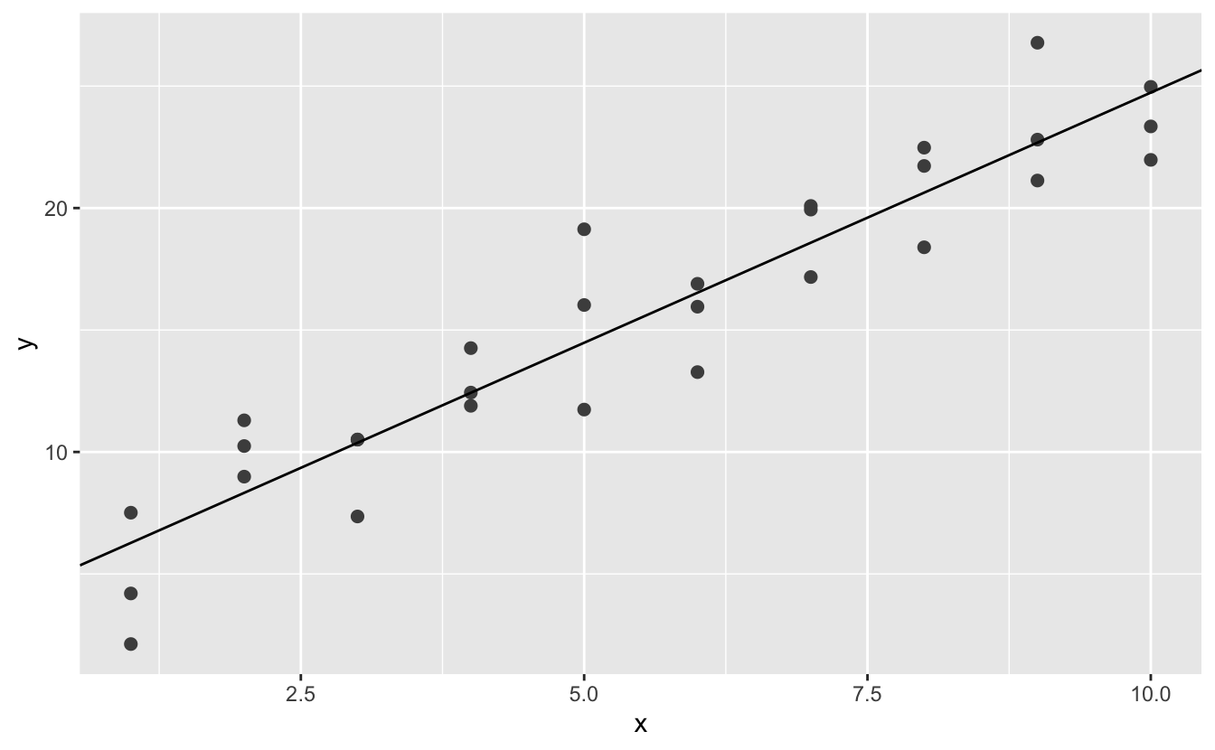
Don't worry likewise much about the details of how optim() works. Information technology'southward the intuition that's important here. If yous have a function that defines the altitude between a model and a dataset, an algorithm that can minimise that distance by modifying the parameters of the model, you tin can find the best model. The slap-up thing almost this approach is that it will work for any family unit of models that you lot can write an equation for.
There'southward one more than approach that we can utilize for this model, because it'due south a special case of a broader family unit: linear models. A linear model has the full general class y = a_1 + a_2 * x_1 + a_3 * x_2 + ... + a_n * x_(north - 1). So this simple model is equivalent to a full general linear model where northward is 2 and x_1 is x. R has a tool specifically designed for plumbing fixtures linear models called lm(). lm() has a special mode to specify the model family: formulas. Formulas look like y ~ x, which lm() will translate to a role like y = a_1 + a_2 * x. Nosotros tin can fit the model and look at the output:
sim1_mod <- lm ( y ~ x, information = sim1 ) coef ( sim1_mod ) #> (Intercept) 10 #> iv.220822 2.051533 These are exactly the aforementioned values we got with optim()! Backside the scenes lm() doesn't employ optim() but instead takes reward of the mathematical construction of linear models. Using some connections between geometry, calculus, and linear algebra, lm() actually finds the closest model in a unmarried step, using a sophisticated algorithm. This approach is both faster, and guarantees that there is a global minimum.
Exercises
-
One downside of the linear model is that information technology is sensitive to unusual values because the distance incorporates a squared term. Fit a linear model to the faux data below, and visualise the results. Rerun a few times to generate different simulated datasets. What practise you discover about the model?
sim1a <- tibble ( x = rep ( i : 10, each = 3 ), y = x * one.5 + vi + rt ( length ( x ), df = 2 ) ) -
One fashion to brand linear models more than robust is to use a different altitude measure. For instance, instead of root-mean-squared altitude, you could apply mean-absolute distance:
measure_distance <- function ( modern, data ) { diff <- data $ y - model1 ( modern, data ) mean ( abs ( diff ) ) }Employ
optim()to fit this model to the imitation data in a higher place and compare it to the linear model. -
1 challenge with performing numerical optimisation is that information technology's only guaranteed to find 1 local optimum. What'due south the problem with optimising a three parameter model similar this?
model1 <- function ( a, data ) { a [ ane ] + data $ x * a [ ii ] + a [ 3 ] }
Visualising models
For elementary models, like the one above, you lot can figure out what pattern the model captures by carefully studying the model family and the fitted coefficients. And if you ever take a statistics course on modelling, yous're likely to spend a lot of time doing only that. Here, nonetheless, nosotros're going to take a different tack. We're going to focus on understanding a model by looking at its predictions. This has a large advantage: every type of predictive model makes predictions (otherwise what use would it be?) so we tin can use the same gear up of techniques to understand any type of predictive model.
Information technology's also useful to see what the model doesn't capture, the and so-called residuals which are left after subtracting the predictions from the data. Residuals are powerful considering they allow united states of america to use models to remove striking patterns so nosotros can study the subtler trends that remain.
Predictions
To visualise the predictions from a model, we start past generating an evenly spaced grid of values that covers the region where our data lies. The easiest way to do that is to employ modelr::data_grid(). Its first argument is a information frame, and for each subsequent argument it finds the unique variables and and so generates all combinations:
filigree <- sim1 %>% data_grid ( ten ) grid #> # A tibble: 10 x 1 #> x #> <int> #> ane 1 #> 2 2 #> 3 3 #> 4 four #> 5 five #> half-dozen 6 #> # … with iv more than rows (This volition go more interesting when we showtime to add together more variables to our model.)
Next we add predictions. We'll utilise modelr::add_predictions() which takes a information frame and a model. It adds the predictions from the model to a new column in the data frame:
filigree <- filigree %>% add_predictions ( sim1_mod ) filigree #> # A tibble: 10 x 2 #> x pred #> <int> <dbl> #> 1 i 6.27 #> 2 two 8.32 #> iii 3 10.4 #> 4 four 12.4 #> 5 5 14.5 #> six half dozen 16.5 #> # … with four more rows (You lot can too use this office to add predictions to your original dataset.)
Next, we plot the predictions. You might wonder about all this extra piece of work compared to merely using geom_abline(). But the reward of this approach is that information technology volition work with whatsoever model in R, from the simplest to the nigh complex. You're only limited by your visualisation skills. For more ideas almost how to visualise more than complex model types, you lot might try http://vita.had.co.nz/papers/model-vis.html.

Residuals
The flip-side of predictions are residuals. The predictions tells you the pattern that the model has captured, and the residuals tell you what the model has missed. The residuals are just the distances between the observed and predicted values that we computed higher up.
Nosotros add residuals to the data with add_residuals(), which works much like add_predictions(). Note, nonetheless, that we use the original dataset, not a manufactured grid. This is because to compute residuals we demand actual y values.
sim1 <- sim1 %>% add_residuals ( sim1_mod ) sim1 #> # A tibble: 30 ten 3 #> x y resid #> <int> <dbl> <dbl> #> 1 1 four.20 -2.07 #> two i seven.51 one.24 #> 3 1 2.13 -4.15 #> 4 2 viii.99 0.665 #> 5 2 10.2 1.92 #> 6 2 11.3 2.97 #> # … with 24 more rows There are a few different means to understand what the residuals tell us nigh the model. Ane way is to simply draw a frequency polygon to aid us understand the spread of the residuals:

This helps you calibrate the quality of the model: how far abroad are the predictions from the observed values? Note that the average of the remainder will always be 0.
Yous'll ofttimes desire to recreate plots using the residuals instead of the original predictor. You lot'll come across a lot of that in the next chapter.

This looks like random noise, suggesting that our model has done a practiced job of capturing the patterns in the dataset.
Exercises
-
Instead of using
lm()to fit a straight line, yous can useloess()to fit a shine curve. Repeat the process of model plumbing equipment, grid generation, predictions, and visualisation onsim1usingloess()instead oflm(). How does the upshot compare togeom_smooth()? -
add_predictions()is paired withgather_predictions()andspread_predictions(). How practise these three functions differ? -
What does
geom_ref_line()do? What packet does it come from? Why is displaying a reference line in plots showing residuals useful and important? -
Why might y'all want to expect at a frequency polygon of absolute residuals? What are the pros and cons compared to looking at the raw residuals?
Formulas and model families
Yous've seen formulas earlier when using facet_wrap() and facet_grid(). In R, formulas provide a general mode of getting "special behaviour". Rather than evaluating the values of the variables right away, they capture them and then they tin be interpreted by the role.
The majority of modelling functions in R employ a standard conversion from formulas to functions. You've seen one simple conversion already: y ~ x is translated to y = a_1 + a_2 * x. If you want to run across what R actually does, you can use the model_matrix() function. It takes a information frame and a formula and returns a tibble that defines the model equation: each cavalcade in the output is associated with one coefficient in the model, the office is always y = a_1 * out1 + a_2 * out_2. For the simplest example of y ~ x1 this shows usa something interesting:
df <- tribble ( ~ y, ~ x1, ~ x2, iv, two, five, five, 1, 6 ) model_matrix ( df, y ~ x1 ) #> # A tibble: ii x ii #> `(Intercept)` x1 #> <dbl> <dbl> #> 1 i ii #> 2 1 1 The way that R adds the intercept to the model is just past having a column that is full of ones. Past default, R will e'er add this cavalcade. If you don't want, you lot need to explicitly drop it with -1:
model_matrix ( df, y ~ x1 - 1 ) #> # A tibble: 2 ten i #> x1 #> <dbl> #> 1 ii #> 2 1 The model matrix grows in an unsurprising way when you add more variables to the the model:
model_matrix ( df, y ~ x1 + x2 ) #> # A tibble: ii x 3 #> `(Intercept)` x1 x2 #> <dbl> <dbl> <dbl> #> 1 1 two five #> 2 one 1 half dozen This formula notation is sometimes chosen "Wilkinson-Rogers notation", and was initially described in Symbolic Description of Factorial Models for Analysis of Variance, past G. N. Wilkinson and C. E. Rogers https://www.jstor.org/stable/2346786. It's worth digging upwards and reading the original paper if you'd like to understand the full details of the modelling algebra.
The following sections expand on how this formula notation works for chiselled variables, interactions, and transformation.
Categorical variables
Generating a function from a formula is straight forward when the predictor is continuous, but things get a fleck more complicated when the predictor is chiselled. Imagine you lot have a formula like y ~ sex, where sexual activity could either exist male or female person. It doesn't brand sense to convert that to a formula like y = x_0 + x_1 * sexual practice because sex isn't a number - you lot can't multiply it! Instead what R does is convert it to y = x_0 + x_1 * sex_male where sex_male is one if sex is male and zippo otherwise:
df <- tribble ( ~ sex, ~ response, "male", 1, "female", 2, "male", i ) model_matrix ( df, response ~ sexual activity ) #> # A tibble: 3 x ii #> `(Intercept)` sexmale #> <dbl> <dbl> #> 1 1 1 #> 2 1 0 #> 3 1 1 Y'all might wonder why R also doesn't create a sexfemale column. The problem is that would create a column that is perfectly predictable based on the other columns (i.e.sexfemale = ane - sexmale). Unfortunately the exact details of why this is a trouble is beyond the telescopic of this book, but basically it creates a model family unit that is besides flexible, and will have infinitely many models that are equally close to the information.
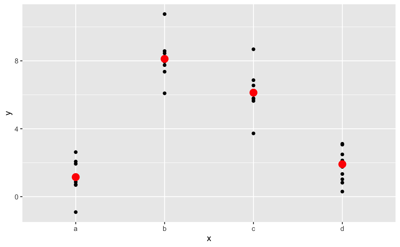
Fortunately, however, if yous focus on visualising predictions you don't need to worry nearly the exact parameterisation. Permit's wait at some information and models to make that concrete. Hither's the sim2 dataset from modelr:

We tin can fit a model to it, and generate predictions:
mod2 <- lm ( y ~ x, information = sim2 ) grid <- sim2 %>% data_grid ( x ) %>% add_predictions ( mod2 ) grid #> # A tibble: 4 x 2 #> x pred #> <chr> <dbl> #> 1 a i.15 #> 2 b viii.12 #> 3 c 6.thirteen #> 4 d ane.91 Effectively, a model with a chiselled x will predict the mean value for each category. (Why? Considering the mean minimises the root-mean-squared distance.) That's easy to see if we overlay the predictions on summit of the original data:
You can't make predictions about levels that you didn't notice. Sometimes y'all'll do this past blow so it's expert to recognise this error message:
tibble (x = "east" ) %>% add_predictions ( mod2 ) #> Error in model.frame.default(Terms, newdata, na.action = na.action, xlev = object$xlevels): factor x has new level east Interactions (continuous and categorical)
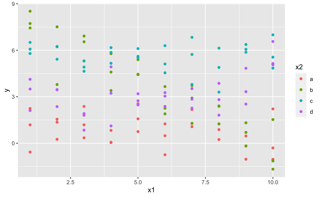
What happens when you combine a continuous and a categorical variable? sim3 contains a categorical predictor and a continuous predictor. Nosotros tin can visualise it with a uncomplicated plot:
There are two possible models you could fit to this information:
mod1 <- lm ( y ~ x1 + x2, data = sim3 ) mod2 <- lm ( y ~ x1 * x2, data = sim3 ) When yous add together variables with +, the model will gauge each effect independent of all the others. It's possible to fit the so-called interaction past using *. For example, y ~ x1 * x2 is translated to y = a_0 + a_1 * x1 + a_2 * x2 + a_12 * x1 * x2. Notation that whenever yous apply *, both the interaction and the private components are included in the model.
To visualise these models we need two new tricks:
-
We have two predictors, so we need to give
data_grid()both variables. It finds all the unique values ofx1andx2and then generates all combinations. -
To generate predictions from both models simultaneously, we can use
gather_predictions()which adds each prediction equally a row. The complement ofgather_predictions()isspread_predictions()which adds each prediction to a new column.
Together this gives us:
grid <- sim3 %>% data_grid ( x1, x2 ) %>% gather_predictions ( mod1, mod2 ) filigree #> # A tibble: 80 ten iv #> model x1 x2 pred #> <chr> <int> <fct> <dbl> #> ane mod1 ane a 1.67 #> 2 mod1 1 b four.56 #> 3 mod1 1 c half-dozen.48 #> four mod1 1 d four.03 #> v mod1 two a one.48 #> 6 mod1 2 b 4.37 #> # … with 74 more rows Nosotros tin can visualise the results for both models on ane plot using facetting:
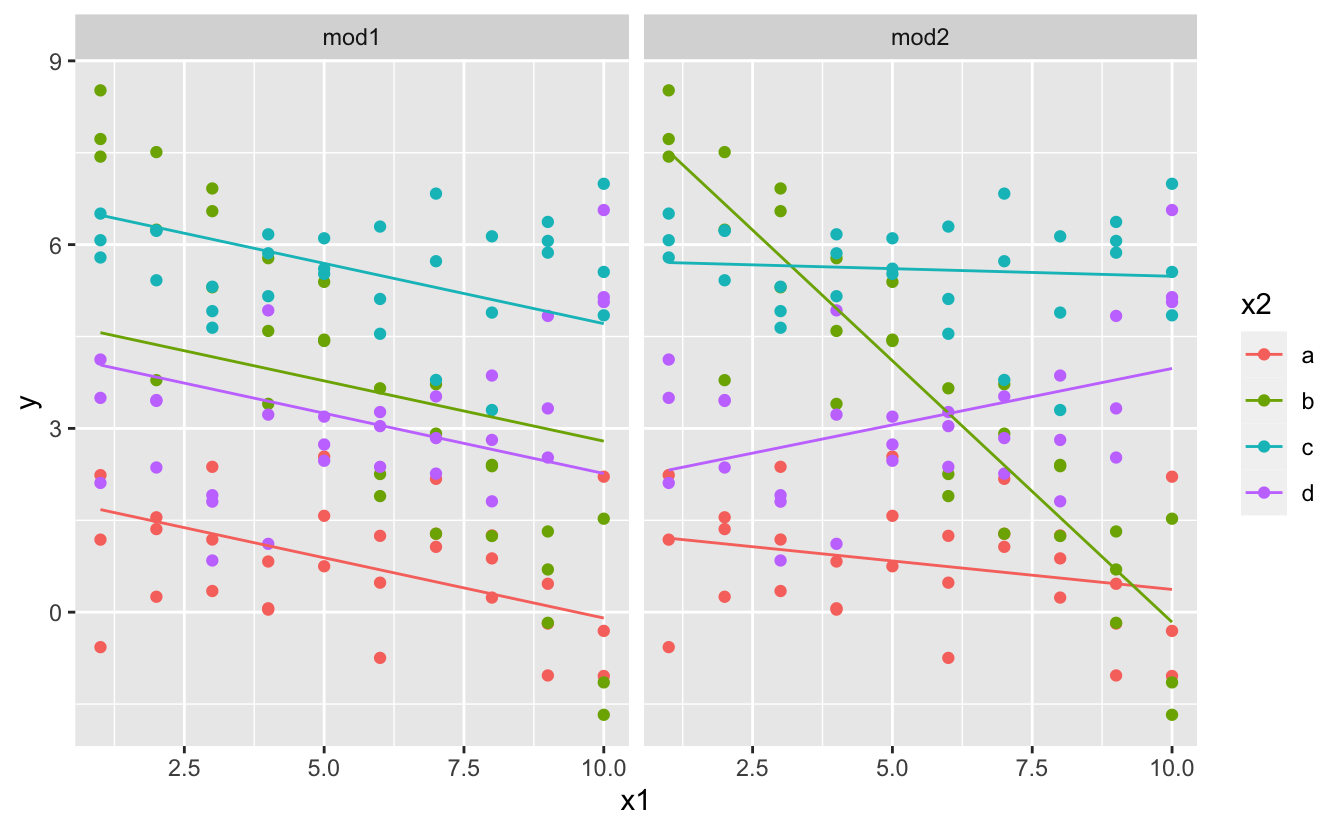
Note that the model that uses + has the same slope for each line, simply unlike intercepts. The model that uses * has a unlike slope and intercept for each line.
Which model is improve for this information? We tin can take look at the residuals. Here I've facetted by both model and x2 because it makes information technology easier to see the pattern within each group.
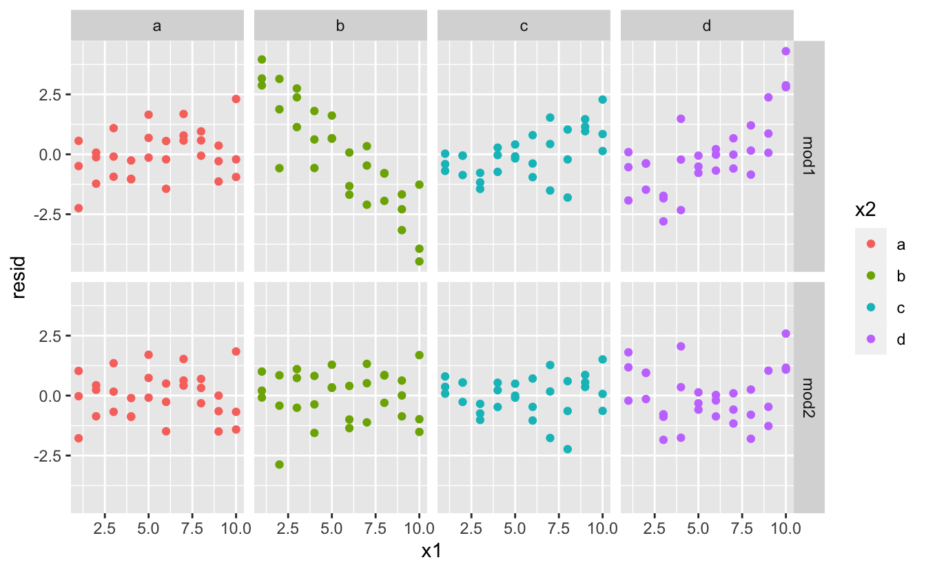
There is little obvious pattern in the residuals for mod2. The residuals for mod1 show that the model has clearly missed some pattern in b, and less so, simply still present is design in c, and d. You might wonder if there's a precise way to tell which of mod1 or mod2 is better. At that place is, but it requires a lot of mathematical background, and we don't really care. Hither, we're interested in a qualitative cess of whether or non the model has captured the pattern that nosotros're interested in.
Interactions (two continuous)
Let's take a look at the equivalent model for ii continuous variables. Initially things go along almost identically to the previous example:
mod1 <- lm ( y ~ x1 + x2, data = sim4 ) mod2 <- lm ( y ~ x1 * x2, data = sim4 ) grid <- sim4 %>% data_grid ( x1 = seq_range ( x1, 5 ), x2 = seq_range ( x2, 5 ) ) %>% gather_predictions ( mod1, mod2 ) grid #> # A tibble: 50 ten 4 #> model x1 x2 pred #> <chr> <dbl> <dbl> <dbl> #> 1 mod1 -1 -1 0.996 #> 2 mod1 -1 -0.5 -0.395 #> 3 mod1 -1 0 -1.79 #> 4 mod1 -one 0.five -three.xviii #> five mod1 -1 one -4.57 #> six mod1 -0.5 -1 1.91 #> # … with 44 more rows Note my use of seq_range() within data_grid(). Instead of using every unique value of x, I'grand going to utilize a regularly spaced grid of 5 values betwixt the minimum and maximum numbers. It's probably not super important here, but information technology's a useful technique in general. There are two other useful arguments to seq_range():
-
pretty = Truthfulwill generate a "pretty" sequence, i.east. something that looks dainty to the human being eye. This is useful if you desire to produce tables of output:seq_range ( c ( 0.0123, 0.923423 ), n = 5 ) #> [one] 0.0123000 0.2400808 0.4678615 0.6956423 0.9234230 seq_range ( c ( 0.0123, 0.923423 ), n = v, pretty = Truthful ) #> [1] 0.0 0.2 0.4 0.half dozen 0.viii 1.0 -
trim = 0.1will trim off 10% of the tail values. This is useful if the variables have a long tailed distribution and you want to focus on generating values most the center:x1 <- rcauchy ( 100 ) seq_range ( x1, n = five ) #> [one] -115.86934 -83.52130 -51.17325 -18.82520 13.52284 seq_range ( x1, northward = v, trim = 0.ten ) #> [1] -xiii.841101 -8.709812 -3.578522 1.552767 6.684057 seq_range ( x1, n = 5, trim = 0.25 ) #> [1] -ii.17345439 -1.05938856 0.05467728 1.16874312 2.28280896 seq_range ( x1, due north = 5, trim = 0.fifty ) #> [one] -0.7249565 -0.2677888 0.1893788 0.6465465 one.1037141 -
expand = 0.1is in some sense the opposite oftrim()information technology expands the range past x%.x2 <- c ( 0, 1 ) seq_range ( x2, n = 5 ) #> [1] 0.00 0.25 0.50 0.75 1.00 seq_range ( x2, n = 5, aggrandize = 0.10 ) #> [ane] -0.050 0.225 0.500 0.775 1.050 seq_range ( x2, n = v, expand = 0.25 ) #> [1] -0.1250 0.1875 0.5000 0.8125 1.1250 seq_range ( x2, n = 5, aggrandize = 0.50 ) #> [1] -0.250 0.125 0.500 0.875 1.250
Next let'due south endeavor and visualise that model. We accept two continuous predictors, so you tin imagine the model similar a 3d surface. Nosotros could display that using geom_tile():
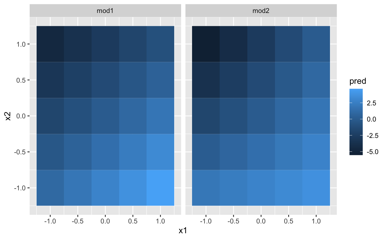
That doesn't suggest that the models are very unlike! But that's partly an illusion: our eyes and brains are not very practiced at accurately comparing shades of colour. Instead of looking at the surface from the elevation, we could wait at it from either side, showing multiple slices:
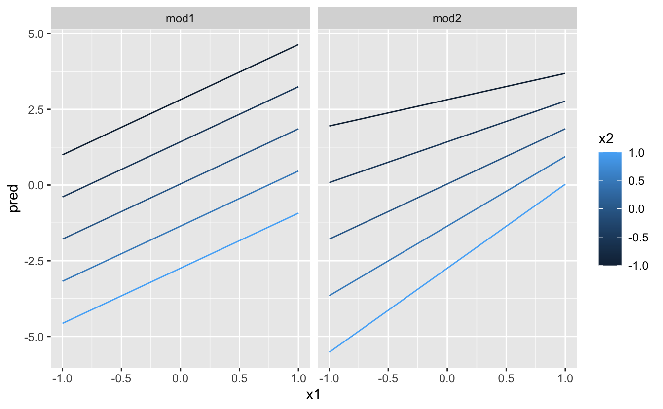
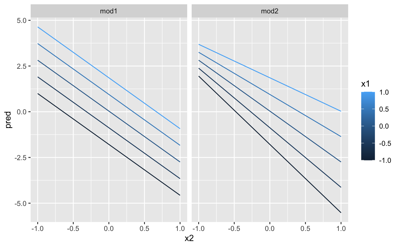
This shows you that interaction between ii continuous variables works basically the same style equally for a categorical and continuous variable. An interaction says that there's non a fixed offset: you need to consider both values of x1 and x2 simultaneously in order to predict y.
You can see that even with just ii continuous variables, coming upwards with good visualisations are hard. But that'south reasonable: you shouldn't expect it volition be easy to empathize how 3 or more than variables simultaneously interact! But once again, nosotros're saved a petty because we're using models for exploration, and you lot tin gradually build up your model over time. The model doesn't have to be perfect, information technology just has to help you reveal a fiddling more about your data.
I spent some time looking at the residuals to see if I could effigy if mod2 did better than mod1. I recollect information technology does, merely it's pretty subtle. You'll have a chance to work on information technology in the exercises.
Transformations
You can also perform transformations inside the model formula. For example, log(y) ~ sqrt(x1) + x2 is transformed to log(y) = a_1 + a_2 * sqrt(x1) + a_3 * x2. If your transformation involves +, *, ^, or -, you lot'll demand to wrap it in I() then R doesn't treat it like part of the model specification. For example, y ~ 10 + I(ten ^ 2) is translated to y = a_1 + a_2 * 10 + a_3 * 10^2. If y'all forget the I() and specify y ~ x ^ two + x, R will compute y ~ x * x + x. x * ten means the interaction of 10 with itself, which is the same as x. R automatically drops redundant variables and then 10 + x become ten, meaning that y ~ x ^ ii + x specifies the part y = a_1 + a_2 * x. That'due south probably not what y'all intended!
Again, if you go confused about what your model is doing, you can always use model_matrix() to see exactly what equation lm() is fitting:
df <- tribble ( ~ y, ~ x, 1, 1, 2, 2, iii, 3 ) model_matrix ( df, y ~ 10 ^ 2 + ten ) #> # A tibble: 3 x 2 #> `(Intercept)` x #> <dbl> <dbl> #> 1 1 i #> 2 one 2 #> three one three model_matrix ( df, y ~ I ( ten ^ 2 ) + x ) #> # A tibble: iii x iii #> `(Intercept)` `I(x^2)` x #> <dbl> <dbl> <dbl> #> one 1 1 one #> 2 1 4 2 #> iii one nine iii Transformations are useful because you can use them to gauge non-linear functions. If you've taken a calculus class, you lot may take heard of Taylor's theorem which says you can estimate whatever polish function with an infinite sum of polynomials. That means yous tin use a polynomial part to get arbitrarily close to a smooth role by fitting an equation like y = a_1 + a_2 * x + a_3 * ten^ii + a_4 * x ^ iii. Typing that sequence by hand is ho-hum, so R provides a helper function: poly():
model_matrix ( df, y ~ poly ( x, 2 ) ) #> # A tibble: 3 x iii #> `(Intercept)` `poly(x, ii)1` `poly(x, 2)2` #> <dbl> <dbl> <dbl> #> 1 1 -7.07e- ane 0.408 #> 2 1 -7.85e-17 -0.816 #> iii 1 seven.07e- one 0.408 However in that location's i major trouble with using poly(): exterior the range of the information, polynomials rapidly shoot off to positive or negative infinity. One safer alternative is to use the natural spline, splines::ns().
library ( splines ) model_matrix ( df, y ~ ns ( ten, 2 ) ) #> # A tibble: 3 x 3 #> `(Intercept)` `ns(x, 2)ane` `ns(x, 2)2` #> <dbl> <dbl> <dbl> #> 1 1 0 0 #> 2 1 0.566 -0.211 #> 3 1 0.344 0.771 Let's run into what that looks like when nosotros try and approximate a non-linear function:
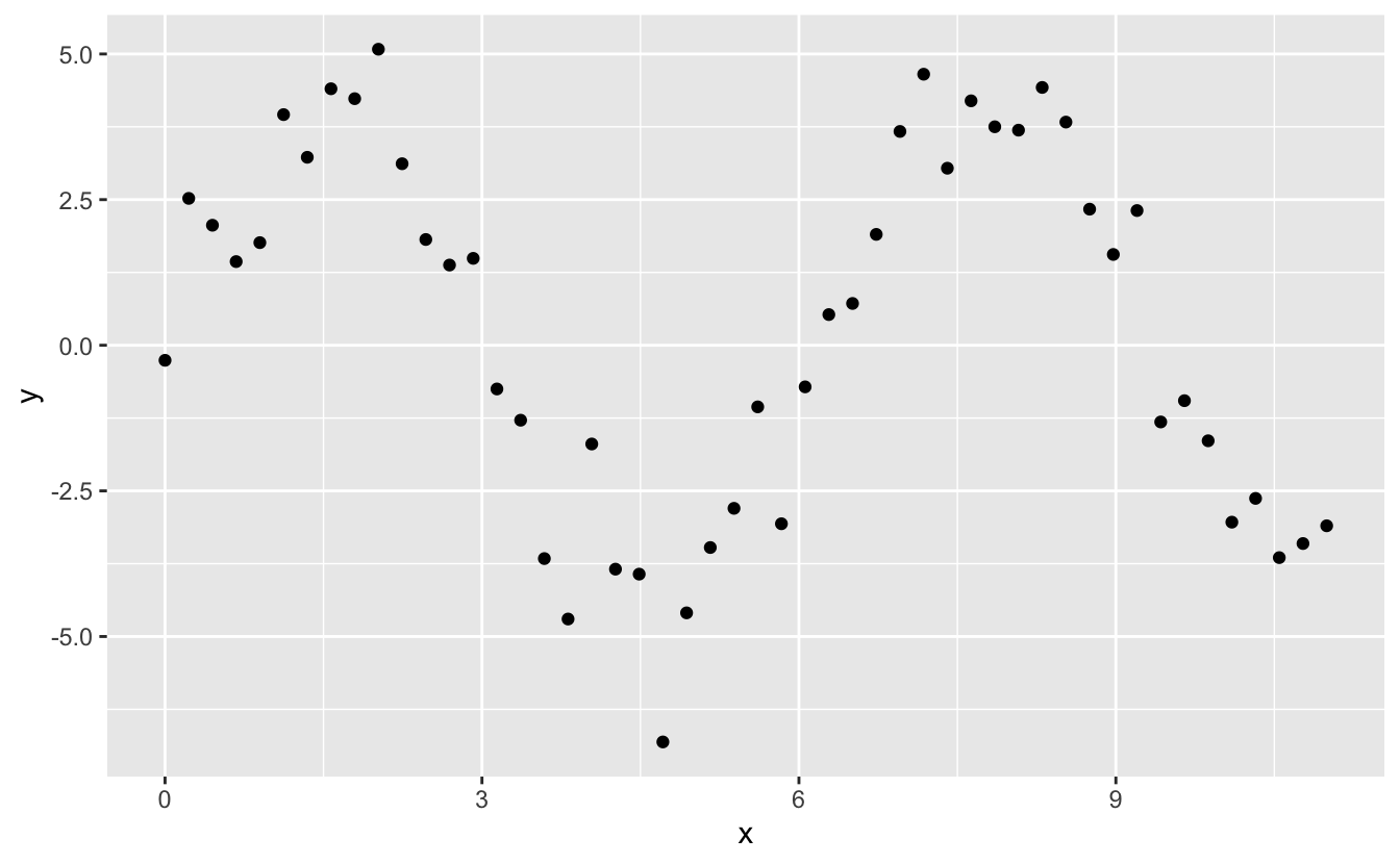
I'1000 going to fit v models to this data.
mod1 <- lm ( y ~ ns ( x, 1 ), information = sim5 ) mod2 <- lm ( y ~ ns ( x, ii ), data = sim5 ) mod3 <- lm ( y ~ ns ( ten, 3 ), information = sim5 ) mod4 <- lm ( y ~ ns ( x, 4 ), data = sim5 ) mod5 <- lm ( y ~ ns ( x, five ), information = sim5 ) grid <- sim5 %>% data_grid (10 = seq_range ( x, n = l, expand = 0.1 ) ) %>% gather_predictions ( mod1, mod2, mod3, mod4, mod5, .pred = "y" ) ggplot ( sim5, aes ( x, y ) ) + geom_point ( ) + geom_line (information = grid, colour = "red" ) + facet_wrap ( ~ model ) 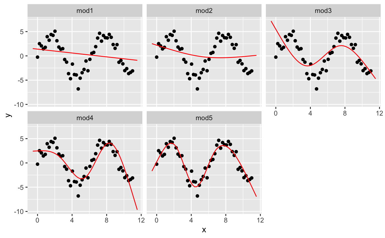
Detect that the extrapolation exterior the range of the data is clearly bad. This is the downside to approximating a function with a polynomial. Only this is a very existent problem with every model: the model tin never tell you if the behaviour is true when you offset extrapolating outside the range of the data that you take seen. Yous must rely on theory and science.
Exercises
-
What happens if you echo the analysis of
sim2using a model without an intercept. What happens to the model equation? What happens to the predictions? -
Utilize
model_matrix()to explore the equations generated for the models I fit tosim3andsim4. Why is*a expert autograph for interaction? -
Using the basic principles, catechumen the formulas in the post-obit 2 models into functions. (Hint: start by converting the categorical variable into 0-1 variables.)
mod1 <- lm ( y ~ x1 + x2, data = sim3 ) mod2 <- lm ( y ~ x1 * x2, data = sim3 ) -
For
sim4, which ofmod1andmod2is amend? I remembermod2does a slightly meliorate chore at removing patterns, but it's pretty subtle. Tin can you come upwards with a plot to support my claim?
Missing values
Missing values obviously can not convey any information nigh the relationship between the variables, and then modelling functions volition drop any rows that comprise missing values. R's default behaviour is to silently drop them, but options(na.action = na.warn) (run in the prerequisites), makes sure you get a alarm.
df <- tribble ( ~ 10, ~ y, one, 2.2, 2, NA, three, three.5, 4, 8.three, NA, 10 ) mod <- lm ( y ~ x, data = df ) #> Warning: Dropping 2 rows with missing values To suppress the warning, set na.activeness = na.exclude:
mod <- lm ( y ~ x, data = df, na.action = na.exclude ) You tin always see exactly how many observations were used with nobs():
Other model families
This chapter has focussed exclusively on the class of linear models, which assume a relationship of the form y = a_1 * x1 + a_2 * x2 + ... + a_n * xn. Linear models additionally assume that the residuals have a normal distribution, which we oasis't talked almost. In that location are a large set of model classes that extend the linear model in various interesting means. Some of them are:
-
Generalised linear models, due east.g.
stats::glm(). Linear models presume that the response is continuous and the error has a normal distribution. Generalised linear models extend linear models to include non-continuous responses (e.k. binary data or counts). They work by defining a distance metric based on the statistical idea of likelihood. -
Generalised additive models, e.grand.
mgcv::gam(), extend generalised linear models to incorporate arbitrary polish functions. That means y'all can write a formula likey ~ southward(x)which becomes an equation likey = f(10)and letgam()estimate what that function is (subject to some smoothness constraints to make the problem tractable). -
Penalised linear models, e.g.
glmnet::glmnet(), add a penalization term to the distance that penalises complex models (equally defined by the distance between the parameter vector and the origin). This tends to make models that generalise better to new datasets from the aforementioned population. -
Robust linear models, east.grand.
MASS::rlm(), tweak the distance to downweight points that are very far away. This makes them less sensitive to the presence of outliers, at the cost of being not quite as good when in that location are no outliers. -
Trees, e.grand.
rpart::rpart(), assail the trouble in a completely different mode than linear models. They fit a slice-wise constant model, splitting the data into progressively smaller and smaller pieces. Trees aren't terribly effective by themselves, merely they are very powerful when used in aggregate by models like random forests (e.g.randomForest::randomForest()) or gradient boosting machines (e.g.xgboost::xgboost.)
These models all piece of work similarly from a programming perspective. One time you've mastered linear models, you should find it piece of cake to master the mechanics of these other model classes. Being a skilled modeller is a mixture of some good general principles and having a big toolbox of techniques. Now that you've learned some general tools and 1 useful grade of models, you lot can go along and acquire more classes from other sources.

Source: https://r4ds.had.co.nz/model-basics.html
Posted by: gibbonsnale1948.blogspot.com
0 Response to "How To Draw A Data Model"
Post a Comment